Updated on:
Tracking Live Video Objects with a Moving Camera: dlib vs KCF vs Re3

Table of contents
Tracking objects in moving-camera footage is harder than with a fixed camera. The camera moves with the person or vehicle carrying it, so blur, occlusion, and sudden scale changes never stop. We tested three trackers, dlib, KCF, and Re3 (Real-Time Recurrent Regression), on six cases. Re3 handled the most, at around 100 FPS, but lost its target when one person passed in front of another. KCF was the most stable in some cases, such as background clutter. Based on our findings, dlib suits static cameras and predictable motion.
Today, the market of public surveillance solutions has a huge niche for computer vision technologies and their implementations. Using these technologies allows us to make a significant step in process automation and data processing, gain meaningful insights from raw data, and improve decision-making. Even though there are some competitors that offer out-of-the box solutions, Oxagile explored one of the most challenging fields of the public surveillance domain, tracking live video objects with a moving camera.
Key takeaways:
- Object tracking becomes more difficult when the camera itself is moving, as changes in perspective, object scale, and background can disrupt tracking accuracy.
- Tracking algorithms differ in how they handle occlusion, changes in object appearance, and camera motion. No single approach, like dlib, KCF, and Re3, performs equally well under all conditions.
- In Oxagile’s practical tests, dlib was better suited to simple tracking scenarios, KCF showed greater stability in several difficult cases, and Re3 delivered around 100 FPS or more with strong results under changing conditions.
- Re3 was the only tested algorithm to reacquire a target after brief full occlusion, but tracking people obscured by other people remained a weakness. This highlights the need to select and adapt tracking methods to actual video conditions.
Why object tracking gets harder with a moving camera
Tracking live video objects with a moving camera in public surveillance is a challenging task due to the following factors:
- Worse quality in comparison to static camera footage
- Motion blur
- Occlusions
- Background clutter
- Constant change of rotation and speed
A major task of a typical video object tracking is aimed at keeping track of a chosen object until the very end of the video or up to the moment the object disappears. The process starts with a bounding box around an object that is given as a set of coordinates. For every next frame of the video, the tracker must locate the object as well as update its internal state so it can continue tracking in the frames that follow.
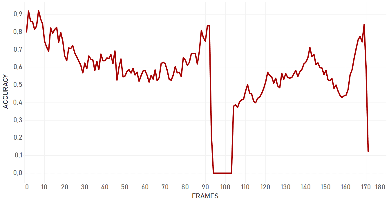
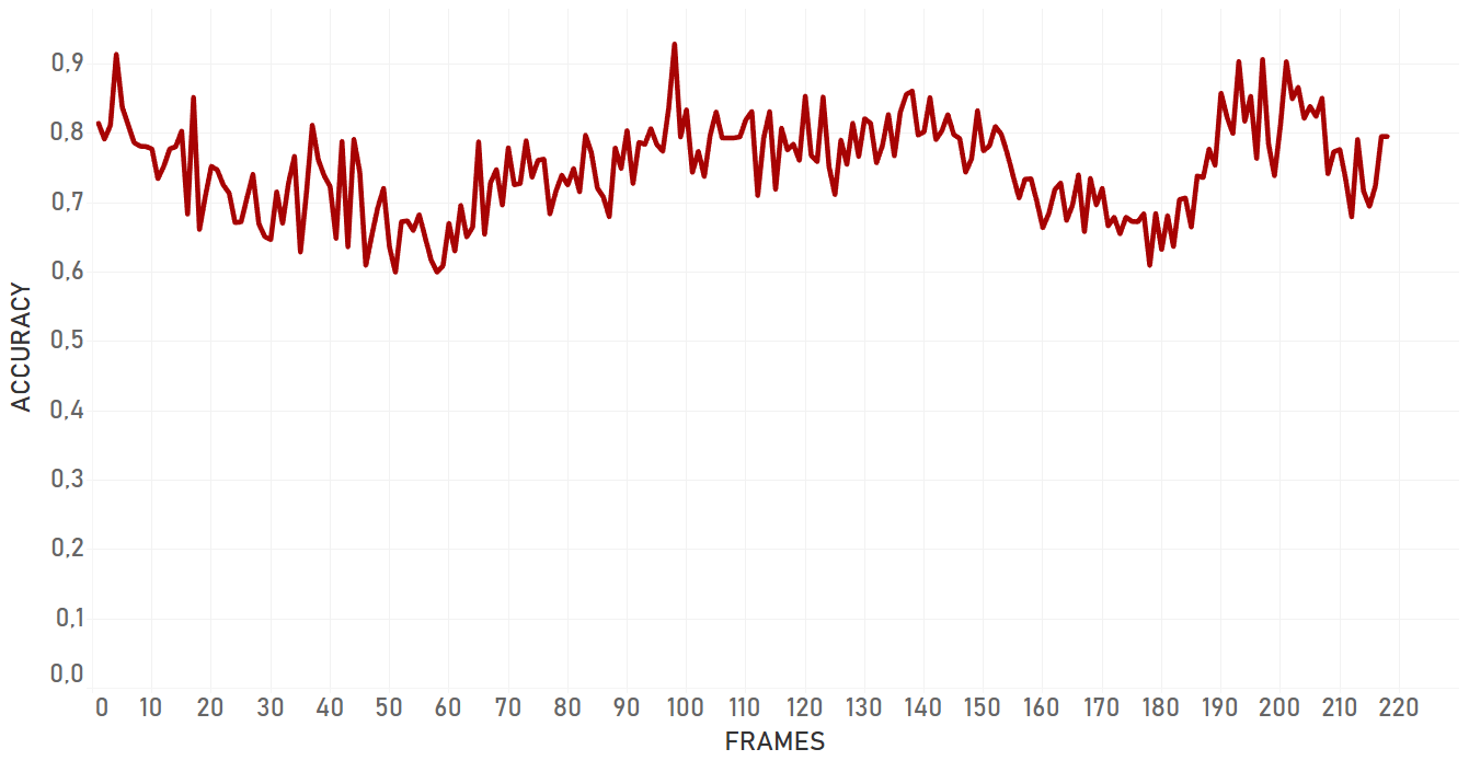
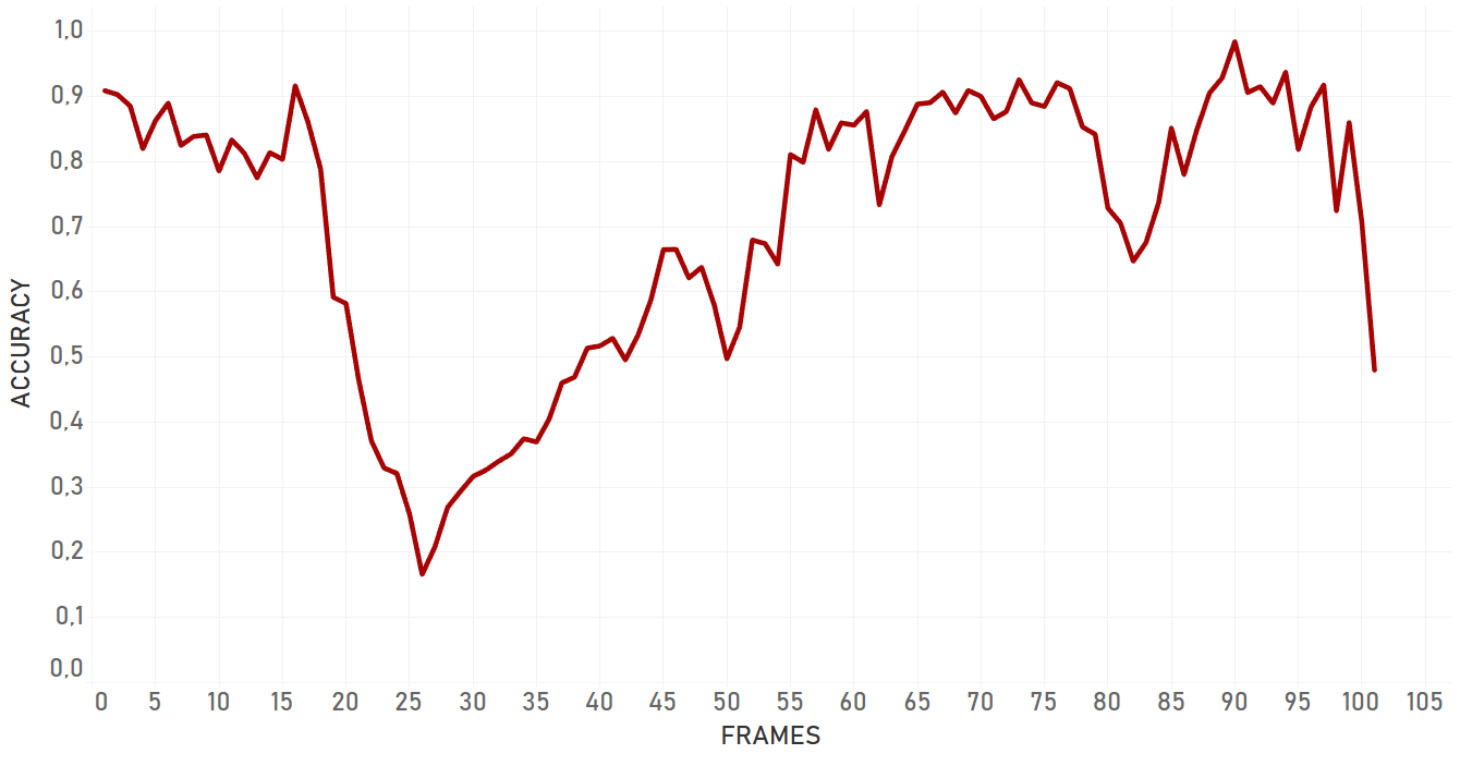
An important goal is to train the algorithm to update the target’s condition to be able to detect its state updates later. To evaluate tracking system performance, we checked Intersection over Union (IoU) metrics that were calculated based on the frame that resulted from tracking performance and manually created a bounding box around the object.
Object tracking methods and their limitations
There are two general high-level tracking approaches.
The first one is to choose an area of interest on the very first frame and then just track it in all the following frames. All the algorithms that we’ll further describe in detail belong to this category.
The second one is to use the algorithms that allow connecting the results of object detection in one line (for example, approaches like Tracking via Generalized Maximum Multi Clique Problem or Graphical Social Topology Model for Multi-Object Tracking).
The majority of tracking approaches are based on the same set of algorithms that were improved and modified for a particular purpose. The basic algorithms are:
 KCF (kernelized correlation filter)
TLD (Tracks, Learns, and Detects)
MOSSE (Minimum Output Sum of Squared Error) filter
Struck (Structured Output Tracking with Kernels)
Median Flow Tracker (this algorithm fails to track objects that move fast or quickly change their appearance)
Most demo videos on the Internet are made using static cameras. Moreover, targeted objects on such recordings are usually located quite far away from the camera, which makes their motions, even the most complex ones, simplified, linear, and more predictable.
If a person or tool on video recording moves, the distance between the camera and the targeted object does not change, they both move at the same speed. Furthermore, in most cases, the object is tracked in an “empty” environment, without any noise, background clutter, or occlusions of the same nature. This creates a new field for research: tracking occluded objects.
On top of this problem, we explore a completely different and complex case that is not covered by any existing algorithm nowadays, processing videos from body cameras. There are several reasons why the complexity of this case makes existing tracking algorithms fail:
- The camera moves together with the person or object it is attached to.
- The trajectory of people and objects around the camera becomes more complex and unpredictable.
- Due to the nature of such recordings, with speed and size of objects changing greatly and quickly, it is difficult to find correct algorithm parameters. This especially concerns the parameters that are responsible for the frequency of state updates. The parameters should be universal to be easily tailored to any case.

Turn live video into actionable intelligence
Put computer vision to work on live camera feeds with object detection, tracking, and automated video analysis tailored to public safety operations.
Object tracking approaches for moving cameras
We tested three object tracking approaches using dlib, KCF, and Re3 to see how each performs when the camera is moving. The comparison focuses on tracking accuracy, stability, and the ability to handle changes in object appearance and position.
DLIB
The dlib tracker is built on the basis of a correlation filter. The correlation algorithm models the object’s appearance after being trained on a sample image patch. In our case, it is given by a user as a bounding box and described by a set of coordinates.
With dlib, it is possible to track objects and update correlation filters or the object’s appearance simultaneously. In order to get a new location of the target on the second and the following frames, we calculate the correlation between the filter and a search window at every next frame, and then find the highest value in the correlation output. Going a bit deeper into the black box of the algorithm, the work of the dlib tracker can be described as follows.
On the very first frame, we extract object features from the area, defined by a manually created bounding box. Initially, all images consist of width and height (commonly known as resolution), and three color channels, which define the color scheme of the picture.
The feature descriptor converts an image to feature vectors of some length. To do that, dlib uses the 31-dimensional version of the HOG (histogram of oriented gradients) feature extraction method [2]. It takes an image, divides it into cells (the cell size is some predefined number), and for each cell, computes a 31-dimensional version of HOG features. It means that for each cell of the image, we have some vector of length, equal to 31, describing this cell.
At the very end, we represent an image as a set of vectors, where shape equals the length of the feature vector (equal to 31), multiplied by the amount of cells fit by width and the amount of cells fit by height.
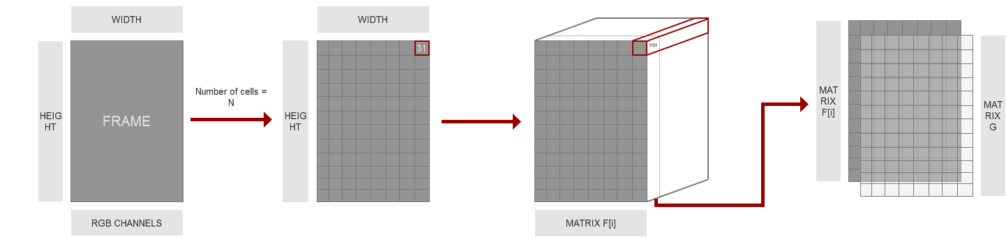
The process of computing this feature vector differs from the standard version of HOG feature extraction, where we are looking at magnitude and direction of the gradient of cell, and there for each image cell we compute the histogram, which contains nine bins corresponding to angles 0, 20, 40 … 160, then concatenate histograms of four neighboring cells, forming a block, into a vector of length 36, normalize the vector, and repeat the process. We will not describe the performance of standard HOG further in detail on this page.
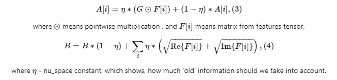
After we extract features of an image, we apply Fourier transform on them. Later it will be necessary to apply the convolution theorem. The reason for such manipulations is to simplify the calculation and make the algorithm less computationally expensive. Here we receive matrices F[i]. By this notation, we will denote in the text below the features that are after applying Fourier transform.
Then we calculate the matrix G in a way to pay more attention to the central area, where the object is located. Calculating the matrix elements involves using the distance values between the point described by the element’s indices and the center of the tensor obtained after some patch processing. We build some sort of mapping between image patch and this matrix, where the values we assign depend on the distance between pixels, corresponding this value and the center of the object. After that, we also apply Fourier transform on this matrix, and take the complex conjugate of the received values. Then we initialize each matrix of filter A (A[i]) by pointwise multiplication of G, obtained above, and the matrix of F[i].
Then we initialize filter B with the formula:

Under the operation of taking the square root from the real or imaginary part of F[i] we mean taking the square root element by element.
Then we make an image pyramid which will help us to understand scale changes on the further frames. In order to do so, we take additional frame patches with certain scale change steps (bigger or smaller) with the same center. Then resize all patches to the size of the original picture. Next we extract HOG features from these patches, and after some transformations, we have a vector of matrices responsible for information about the target on different scale levels, on which we afterwards apply Fourier transform. On the first frame, we initialize scale filters with a slight difference in matrix G filling: we compute it in such a way so that the scale close to the one on the initial frame has the bigger “weight” than other scales. The further we move from the current scale, the less we trust the response.
To find the object’s location and scale on the following frames, we do these procedures:
1. Use the filters we got on the previous frame and features from the current frame to predict the object location by computing the response of the real part of the value:

2. Update the position of the object (the location corresponding to the maximum value in the correlation output indicates the new position of the target). And update the position filters by the following formulas:
In a similar way we are dealing with updating the current scale and scale filters. Here we use the pyramid the following way: one of these patches from the pyramid will have exactly our target in the same scale as we had it on previous frame, and correlation response on this layer will be the highest. The number of this layer will tell us how much the scale of the object has changed. As a final step, we perform tracking as well as for the first step and update the state of the object in the filter. This new state will be compared with the next frame.
Performance tests
| Background clutter case(Background Clutter). The test covers the situation when the person is moving forward in a crowd with other people, being slightly occluded by one of them at a certain moment.
| Appearance changing(3D Rotation). The test covers the situation when the target makes a 3D rotation (the person turns). 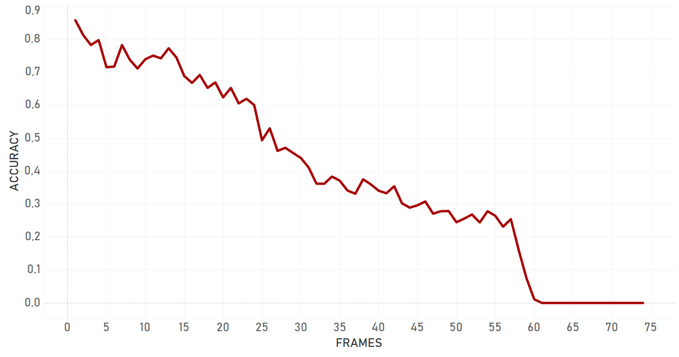 |
| Artist case(Artist). The test covers the situation when the person is static, but the camera moves dynamically. Moreover, the target is small and dark.
| Occlusion by human(Occlusion). The test covers the situation when the person is occluded by another one (occlusion by an object of the same nature).
|
| Appearance changing(Plane Rotation). The test covers the situation when the target is moving in vertical and horizontal scales (the target sits and stands up from the sofa).
| Occlusion by object(Car). The test covers the situation when the target is rapidly hidden behind the part of road construction (occlusion by an object of a different nature).
|
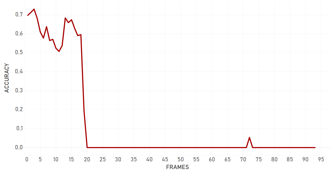
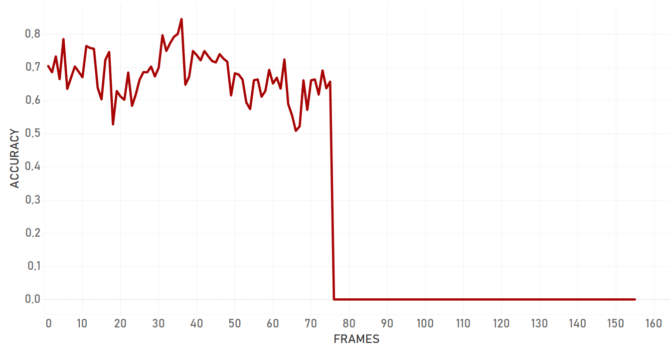
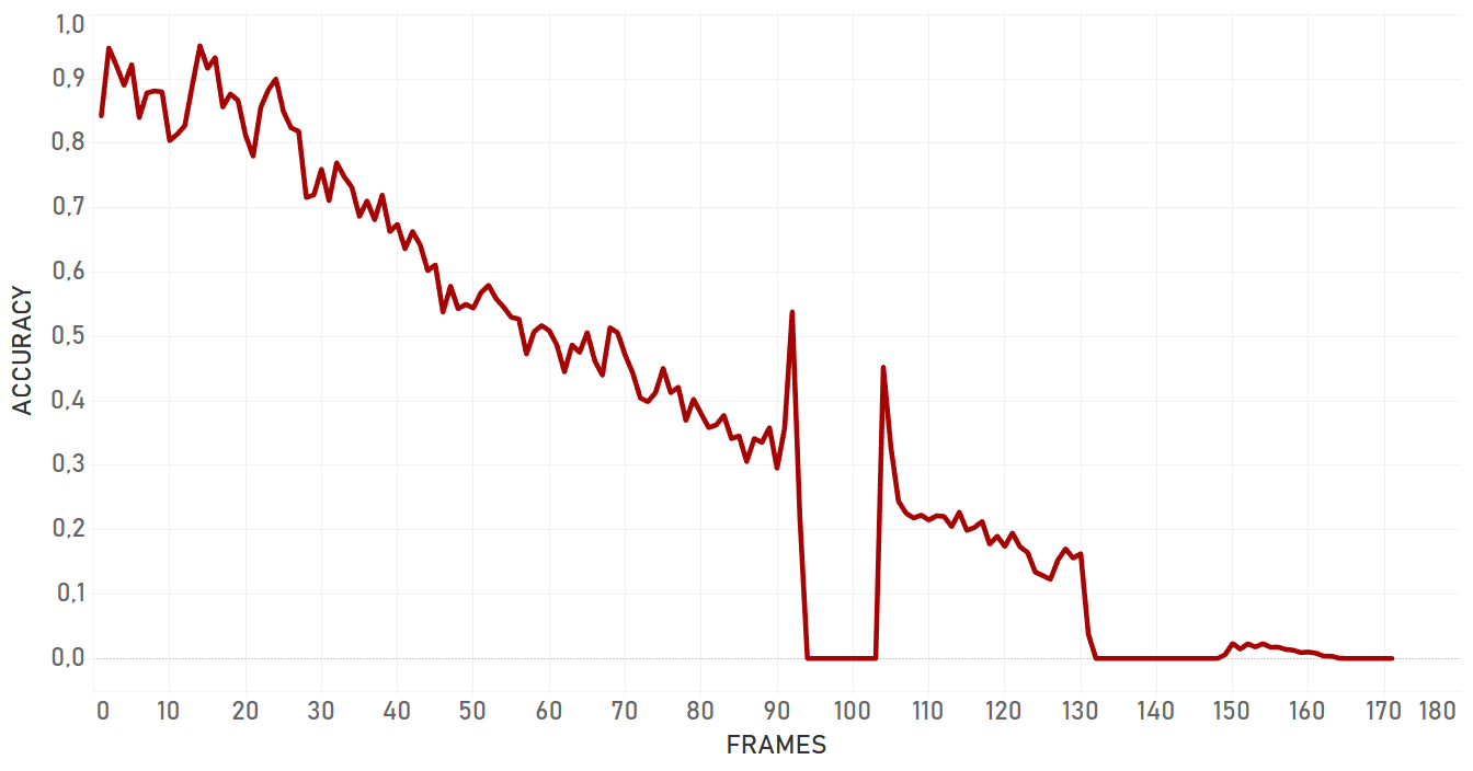
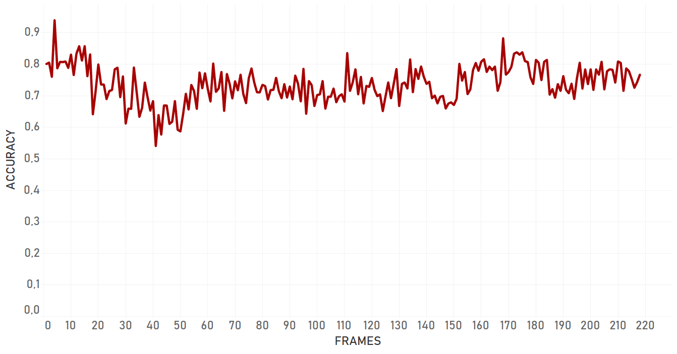
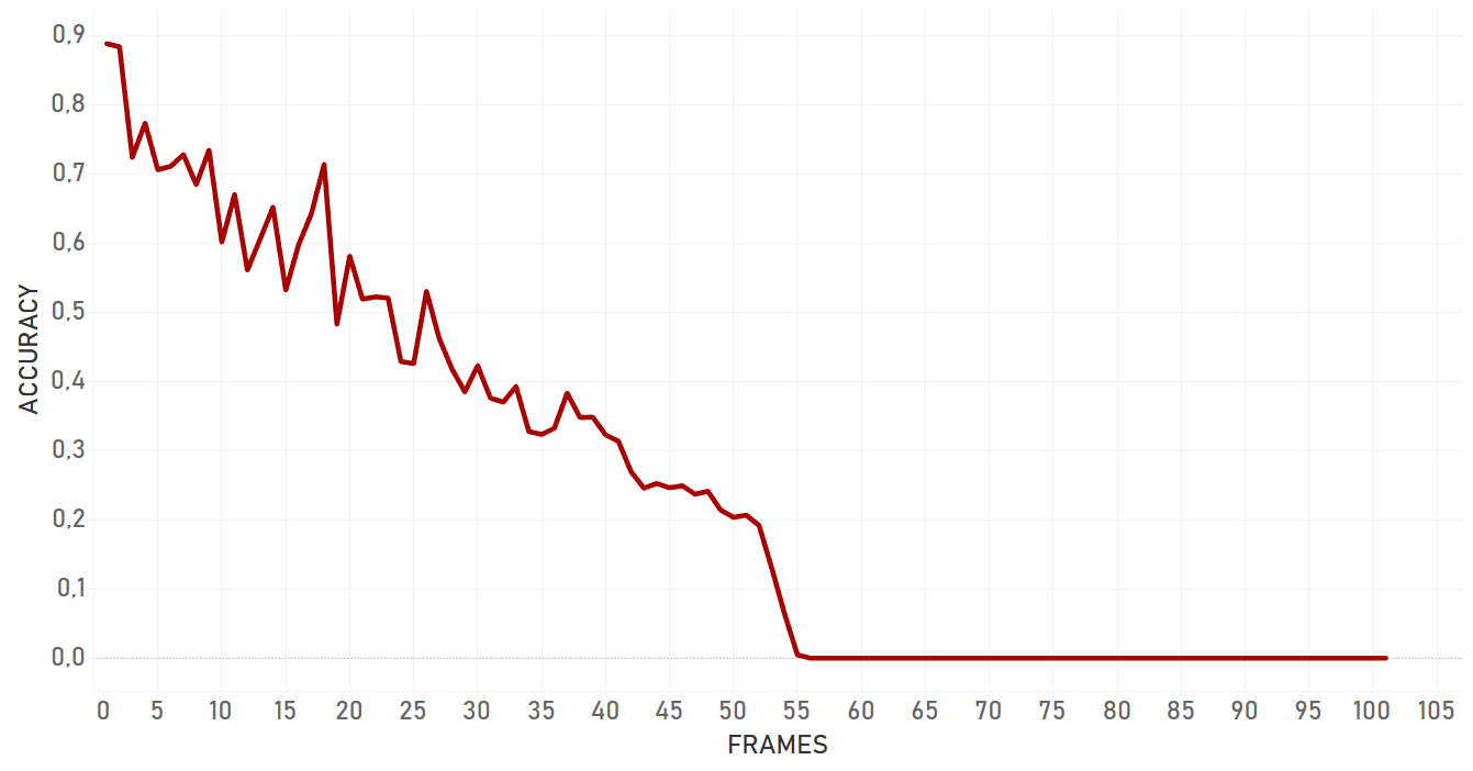
Here we applied intersection over union of ‘right’ bounding box, which we got as a result of tracker work.
Conclusion
Overall, dlib doesn’t show confident and effective performance in case of a moving camera. For the occlusion even with a static camera, it lost the target and switched to the occlusion itself. Also, dlib is not very flexible for the appearance changing, so if the target changes its state, the algorithm will most probably fail.
Dlib is perfect for simple cases and quick analysis, for example, when we need to track objects with predictable and linear trajectories, with no rapid and significant changes in object appearance and environment, no occlusions, and a static camera. Importantly, pure dlib is significantly slower than re3 (which is described further).
KCF
In general, the Kernelized Correlation Filter (KCF) algorithm works similarly to dlib, so we will not describe the process once again. We will highlight the computational differences between the two algorithms, which are almost purely mathematical and can be described by formulas.
I. Bandwidth of Gaussian is dependent on target size
The initial preparation of data for KCF is the same as for dlib: we extract object features (denote them F) from the area under the manually created bounding box. To do so, we use the same 31-dimensional version of HOG features. The difference appears when we create the ‘Gaussian peak’, filling matrix G with some predefined size, making the values dependent on target size.
II. Different approach on Gaussian Correlation
Under Gaussian Correlation we will understand the correlation response map of the Gaussian kernel, expressed by the formula:

In order to find bigger response, we look for the maximal real value between values, as described by the formula:

Note the difference between this formula and (2), used in dlib for computing maximal response.
III. As we use another correlation kernel, formulas for initializing and updating filters will be different
After we make filter B equal to F and compute Gaussian correlation for this frame, passing
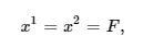
we initialize filters in the following way:
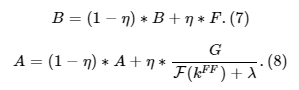
IV. Scale and location finding are done in one step
We build a pyramid and find the best scale with the best correlation output. Then we update the size of the rectangle, and after some geometric transformations (necessary because of repeated image transformations before) we compute the current location of the top left corner of the rectangle. Then we update filters by the formulas A and B provided above (using features of the patch) extracted using a new location and a new scale.
As mentioned above, our goal was to make the tracking algorithm work on videos shot by a moving camera, so it may happen that the scale of the target will change not so much from frame to frame when the object is moving far from the camera, but will change very fast when it will, for example, pass near the camera. At the same time, when the appearance of the object changes dramatically, it may happen that we will get a high response on far pyramid layers, getting fast scale change as a result. In order to find the right balance, we add weighting of each response with a Gaussian at the center of the current scale (that is with zero mean) and some standard deviation, which can be computed from the 3 sigma rule, for example, depending on what exactly the number of layers you want to trust to a greater extent.
Performance tests
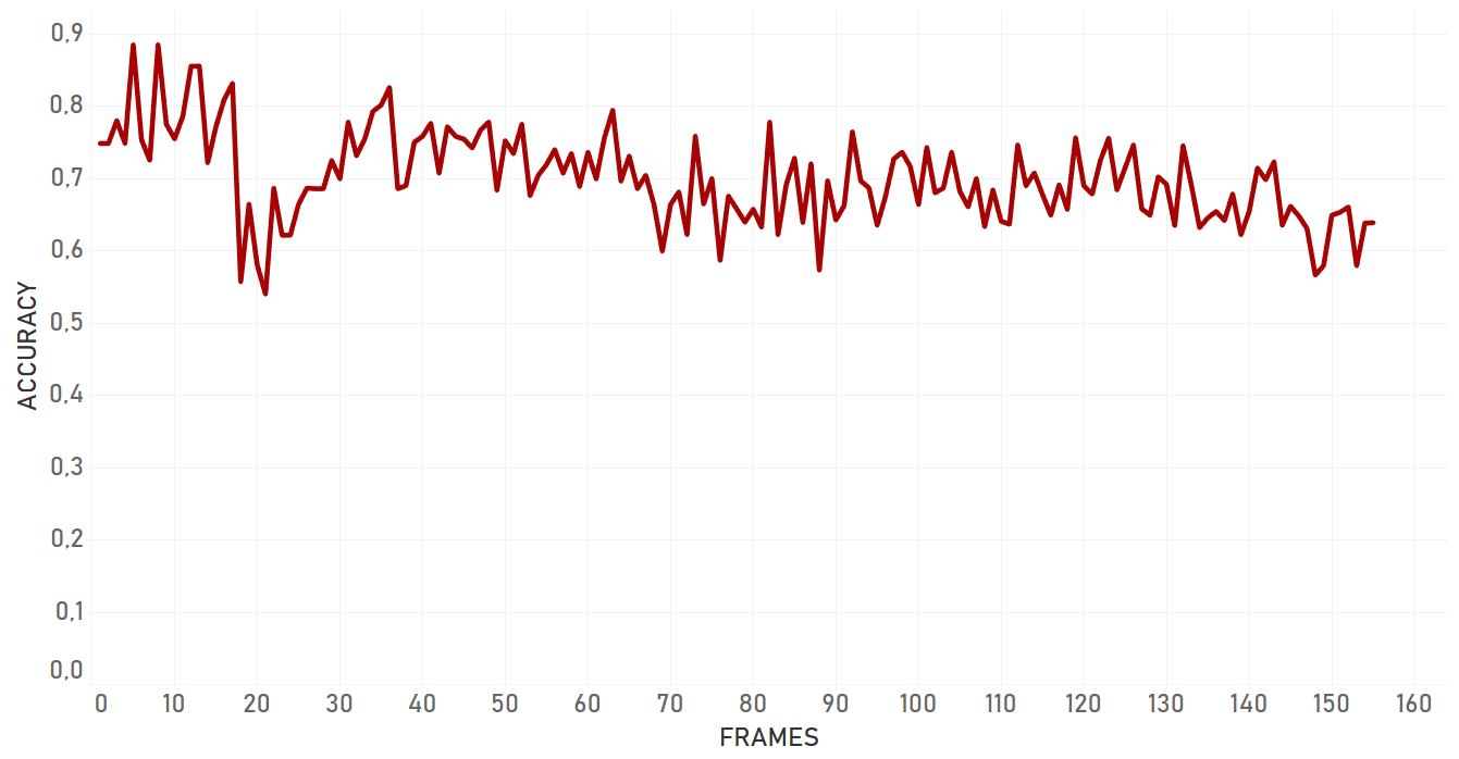
| Background clutter case(Background Clutter). The test covers the situation when the person is moving forward in a crowd of other people, being slightly occluded by one of them at a certain moment.
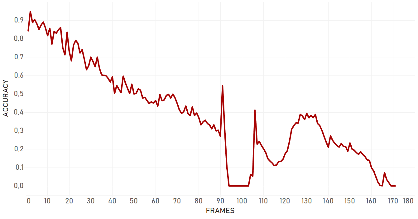
| Appearance changing(3D Rotation). The test covers the situation when the target makes a 3D rotation (the person turns). 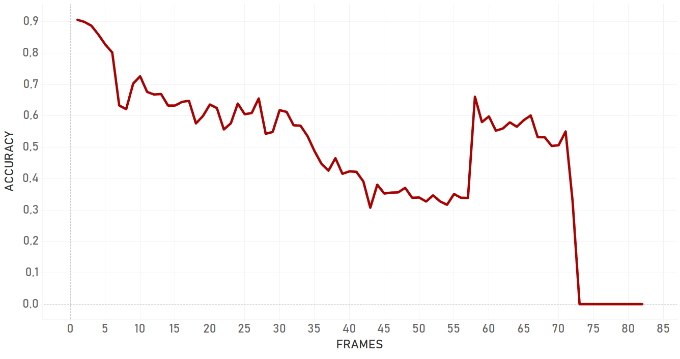 |
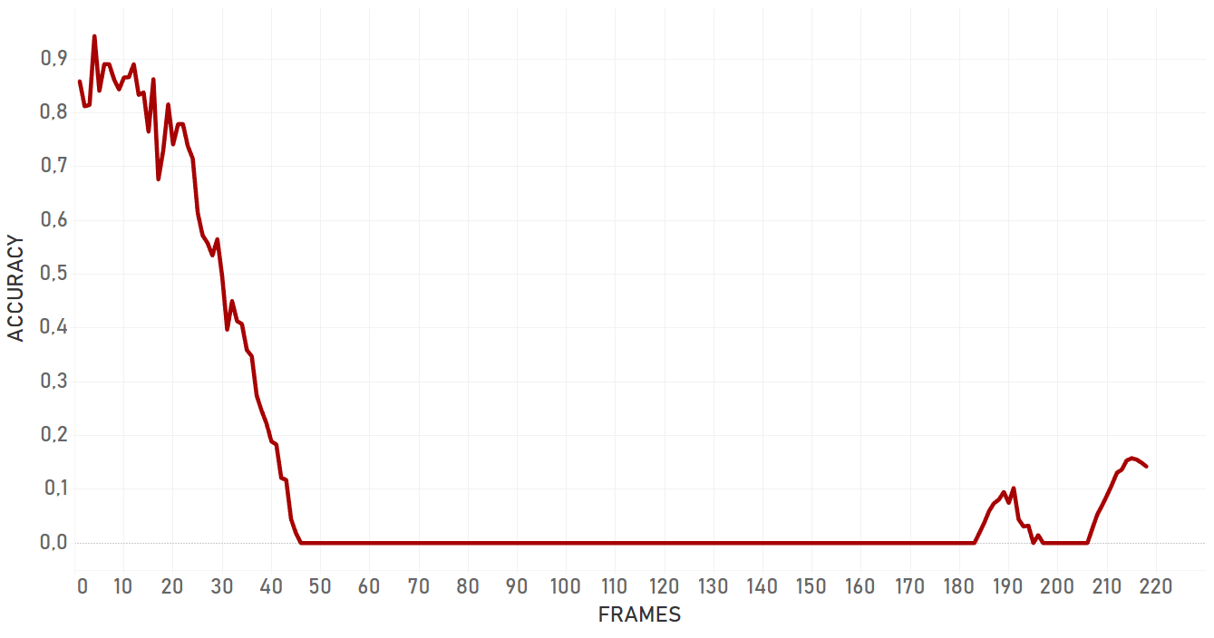
| Artist case(Artist). The test covers the situation when the person is static, but the camera moves dynamically. Moreover, the target is small and dark.
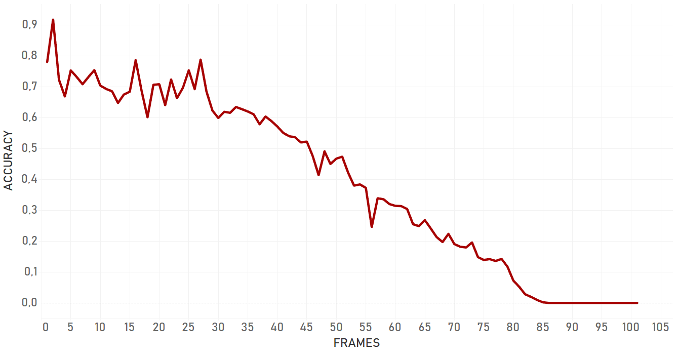
| Occlusion by human(Occlusion). The test covers the situation when the person is occluded by another one (occlusion by an object of the same nature).
|
| Appearance changing(Plane Rotation). The test covers the situation when the target is moving in vertical and horizontal scales (the target sits and stands up from the sofa).
| Occlusion by object(Car). The test covers the situation when the target is rapidly hidden behind the part of road construction (occlusion by an object of a different nature).
|
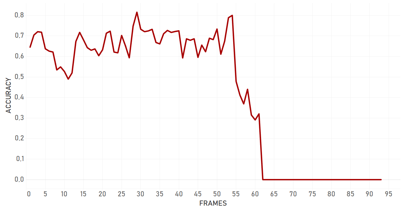
Conclusion
In our tests, KCF performed in a more efficient manner than dlib and showed better results in complex cases. It was more adaptive to the change of appearance, occlusions, and noise of the same nature around of an object, it took more time for KCF to fail. In general, KCF showed significant stability, which is the highest out of all three algorithms we explain here in some cases (for example, the Artist case or the Background clutter case before occlusion).
Re3
Re3 is the Real-Time Recurrent Regression Networks for Visual Tracking of Generic Objects. It is known that recurrent networks often take more iterations to converge and require more hyperparameter selection, and that is the reason they are more difficult to train than feed-forward networks. Re3 present a method of training a recurrent tracking network which translates the image embedding into an output bounding box while simultaneously updating the internal appearance and motion model.
The architecture of the network contains convolution layers, skip connections, recurrent and regression layers. Convolution layers allow us to embed the appearance of the object. The structure of the convolutional network extracts different information from different layers, such as the lowest layers that output features like edge maps, and deeper layers, which are responsible for capturing high-level concepts. Skip connections allow us to recover more fine-grain detail. Recurrent layers remember appearance and motion information, and a regression layer outputs the location of the object.
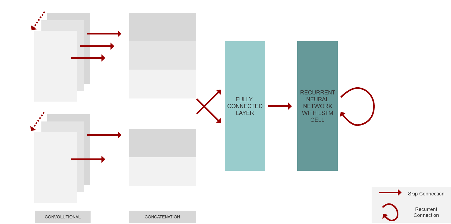
At each step, we feed the network a pair of crops from the image sequence, where the first crop represents the object at the previous frame while the second crop represents the part of the current image centered at the location of the previous frame. Thereby the network can directly compare differences in the two frames and learn how motion affects the image pixels.
Regarding recurrent structure, two-layer, factored LSTM (the visual features are fed to both layers) with peephole connections was chosen. The output and cell state vectors update as the object appearance changes. As each video progresses, the LSTM state is transformed, resulting in many long, thin paths that follow the ordering of the frames in the original video. The second LSTM’s outputs are fed into a fully-connected layer with four output values representing the top left and bottom right corners of the object box in the crop coordinate frame. By regressing these coordinates, we can directly handle size and aspect ratio changes. An L1 loss is used on the outputs to encourage exact matches the ground truth and limit potential drift.
It is also interesting to pay attention to the unrolling during training, as recurrent networks generally take many more iterations to converge than comparable feed-forward networks. This is likely because the inputs are all fed in sequentially, and then one or many outputs and losses are produced. For effective tracking, it is crucial that each input is immediately followed by a corresponding output. So the authors use a training curriculum that begins with few unrolls, and slowly increases the time horizon that the network sees to teach it longer-term relationships. So they initially train the network with only two unrolls and a mini-batch size of 64. After the loss plateaus, they double the number of unrolls and halve the mini-batch size until a maximum unroll of 32 time steps and a mini-batch size of 4.
When training, authors have employed a regime of training that initially relies on ground-truth crops, but over time the network uses its own predictions to generate the next crops. This is because if a network is provided with ground-truth crops at test time, it quickly accumulates more drift than it has ever encountered, and so loses track of the object. This can happen if the recurrent network is trained by feeding ground truth outputs into the future time steps rather than the network’s own predictions. So, initially only the ground truth crops are used, and as the number of unrolls is doubled, the probability of using predicted crops is increased to 0.25, then subsequently to 0.5 and 0.75. So, the random decision is being made over the whole sequence rather than at every step independently.
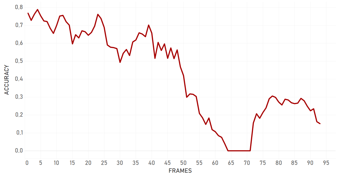
Re3 has showed amazing velocity (around 100 FPS or more) and accuracy performance, with the exception of cases with occlusions by the objects of similar nature. For example, if a person is occluded by another person, there is a high probability that tracker will change the target.
Performance tests
| Background clutter case(Background Clutter). The test covers the situation when the person is moving forward in a crowd among other people, being slightly occluded by one of them at a certain moment.
| Appearance changing(3D Rotation). The test covers the situation when the target makes 3D rotation (person turns). 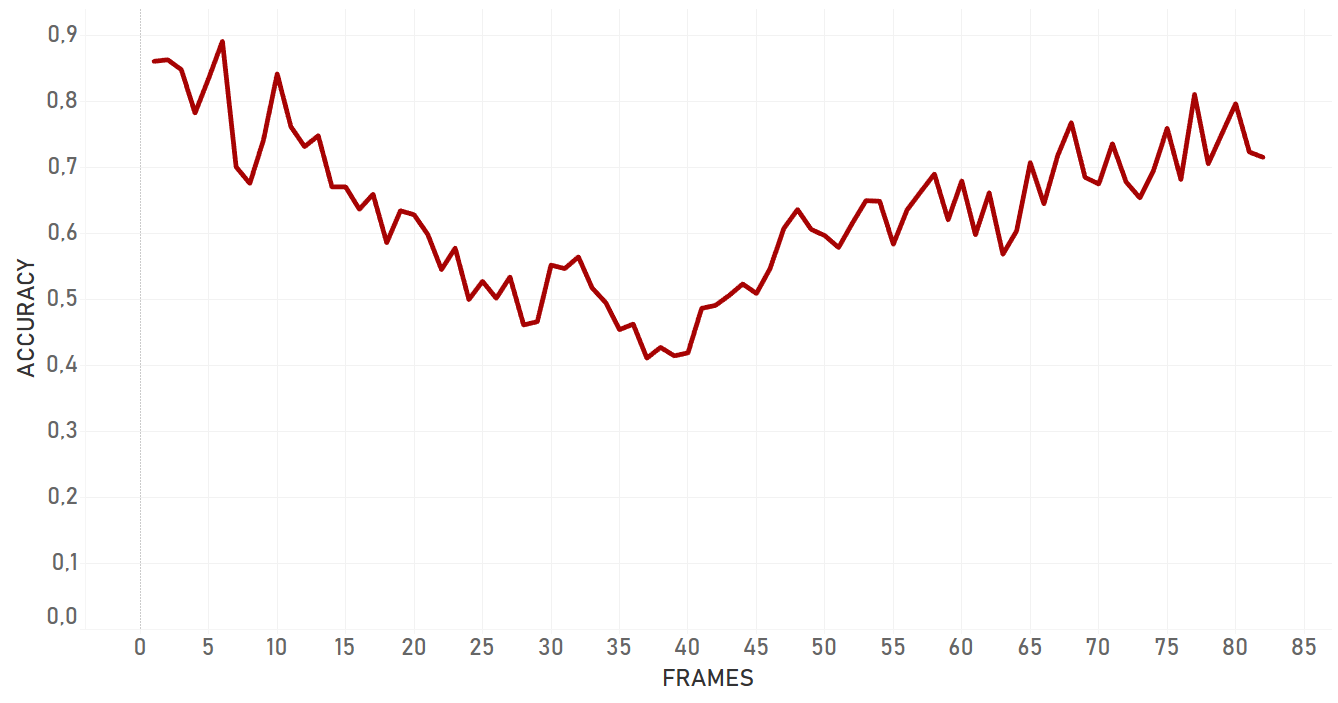 |
| Artist case(Artist). The test covers the situation when the person is static, but the camera moves dynamically. Moreover, the target is small and dark.
| Occlusion by human(Occlusion). The test covers the situation when the person is occluded by another one (occlusion by an object of the same nature).
|
| Appearance changing(Plane Rotation). The test covers the situation when target is moving in vertical and horizontal scales (the target sits and stands up from the sofa).
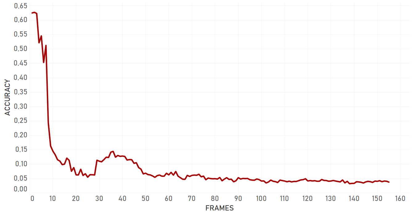
| Occlusion by object(Car). The test covers the situation when the target is rapidly hidden behind the part of road construction (occlusion by an object of a different nature).
|
Conclusion
Re3 showed good results in almost all the cases, including rapid change of object appearance, change of lighting, fast moving, and occlusions. Moreover, it was the only algorithm that was able to catch the object once again following a full occlusion, if the object disappeared for a small amount of time and appeared again approximately in the same area of the frame. In case of a partial occlusion, re3 performed even better and dropped significantly later than dlib or KCF algorithms.
Re3 is perfect for cases with objects that change their appearance, scale, and speed, for full and partial occlusions. The only important weak place of the algorithm that we were able to detect is that its performance significantly drops in case of occlusion with an object of the same nature. In our tests, re3 could not handle this scenario efficiently.
Which tracker fits which footage
| Tracker | Holds up when | Loses the target when | Speed |
|---|---|---|---|
| dlib | The camera is static, and motion is predictable and linear. | The camera moves, anything occludes the target, or the target changes appearance. | Significantly slower than Re3 |
| KCF | Appearance changes, or there is noise around the target. Most stable in the artist case and in background clutter before occlusion. | Complex cases still beat it, but it held on longer than dlib. | No figure given |
| Re3 | Appearance, scale, or speed change fast; full or partial occlusion. It is the only one that found the target again after a short full occlusion. | Another object of the same kind passes in front, for example, one person in front of another. | Around 100 FPS or more |
None of the three wins every case, so the tracker has to match the footage. Hybrid setups often pair a fast tracker like KCF with deep learning that corrects it.
Newer trackers worth knowing
Our tests above cover dlib, KCF, and Re3. The two newer trackers below were not part of those tests.
ByteTrack
One of the latest additions to the tracking toolkit, ByteTrack is known for maintaining high accuracy even in dense scenes with multiple moving targets. It separates detection from tracking, allowing more stable identity preservation.
ByteTrack shines in real-time multi-object tracking scenarios such as crowd monitoring, retail analytics, and sports events. However, it requires strong object detection models as a foundation, and its performance can degrade with inconsistent input quality.
STARK (Spatial-Temporal Transformer Tracker)
STARK leverages transformer-based attention mechanisms to model object relationships across space and time. This allows it to anticipate object motion patterns, handle scale changes, and maintain tracking across abrupt shifts.
While computationally heavier than classical methods, STARK provides exceptional precision in high-complexity scenes and is ideal for use in AI video motion tracking where long-term consistency is required.
What our object tracking research revealed
The main goal of the project was to explore existing opportunities to create a stable and accurate piece of software able to track various objects in moving camera footage. We were able to accomplish the main challenge and achieve fast and accurate performance in poor recording conditions.
Later on, the solution can be used for deeper analysis of videos made by people, body-worn cameras, dashboard cams, and so on. Importantly, the tracking challenge always requires a tailored solution which will take all aspects of the background into consideration, including static or dynamic cameras, the quality of recording, environment conditions, and more. There is no universal and standard solution that will fit all cases and requirements, all of them deserve attention and a detailed observation.
At Oxagile, we are constantly conducting deep research of algorithms and technologies and increase accuracy of our tracking system to improve the overall performance and achieve better results. We are looking to develop custom and high-quality solutions for specific business cases with great attention to the idea of what and why is needed for a product to be effective and valuable.
Tracking footage nobody filmed for analytics?
We build video analytics for body-worn and vehicle cameras, where the scene never holds still.
Sources:
1. Image processing correlation tracker — dlib
2. Object Detection with Discriminatively Trained Part Based Models — IEEE Xplore
3. High-Speed Tracking with Kernelized Correlation Filters — Robots.ox.ac.uk
4. Real-Time Recurrent Regression Networks for Visual Tracking of Generic Objects — arxiv
FAQ
Why do object trackers fail on moving camera footage?
Because the camera moves with the person or vehicle it is attached to. Objects around it change speed, size, and direction quickly, so a tracker tuned on static-camera demos loses them. Motion blur, occlusion, background clutter, and constant rotation make it worse.
Which tracker works best for body camera footage?
In our tests, Re3 handled the most cases, at around 100 FPS, and was the only tracker to find its target again after a short full occlusion. Its weak spot is occlusion by an object of the same kind, such as one person passing in front of another.
How do you measure object tracking accuracy?
We used intersection over union (IoU). The overlap between the box the tracker draws and a box drawn by hand around the same object, frame by frame. The closer the two boxes match, the higher the score.